


The brain is NOT primarily about merely responding to stimuli —
"Whilst part of what we perceive comes through our senses from the object before us, another part (and it may be the larger part) always comes out of our own head."— William James (1890)
[Compare with Lecture 2.2, slide 12]
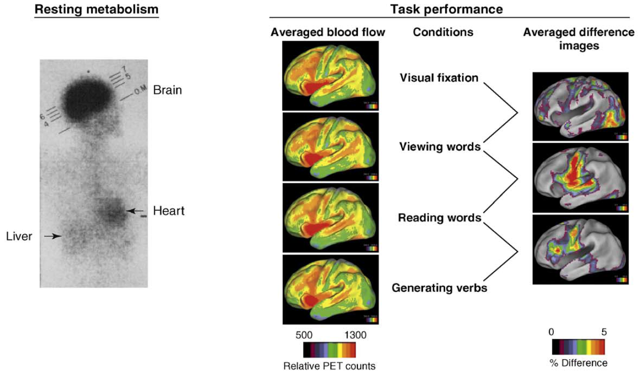
"In the resting state, brain blood flow accounts for 11% of the
cardiac output and brain metabolism accounts for 20% of the energy
consumption of the body, overshadowing the metabolism of other organs such
as the heart, liver and skeletal muscle as shown on the left (above) in
this classic image of whole body glucose consumption. The changes in
regional blood flow associated with task performance are
often no more than 5% of the resting blood flow of the brain from which
they were derived (center) and, hence, only discernable in difference
images averaged across subjects as shown above on the
left right. These modest
modulations in ongoing circulatory and metabolic activity rarely affect the
overall rate of brain blood flow and metabolism during even the most
arousing perceptual and vigorous motor activity."
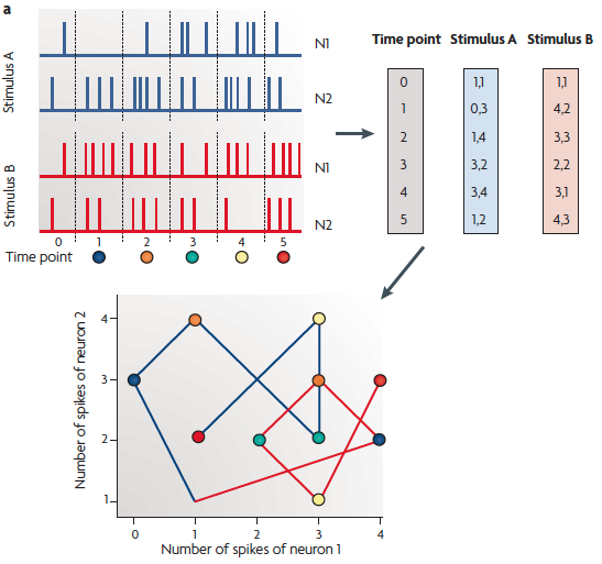
(a) A schematic of a neural trajectory.
The firing pattern of two neurons over five six
time bins constitutes the trajectory of this two-neuron network,
with the number of spikes of each neuron during each time bin
plotted on the axes of a two-dimensional plot. The spikes generated
by two different hypothetical stimuli are represented
in blue and red, and
each produces a different neural trajectory (lower
plot). Importantly, each point on the trajectory can potentially be
used to determine not only which stimulus was presented, but also
how long ago the stimulus was presented (color-coded circles). Thus,
the neural trajectory can inherently encode spatial and temporal
stimulus features. The coordinates represent the number of spikes of
each neuron at each time bin (derived from the upper plot).
Is neural activity better described by SPIKE TRAINS or FIRING RATES?
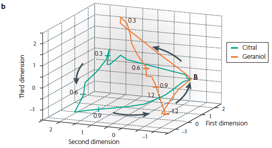
(b) An example of the active trajectory of a population of neurons from the locust antennal lobe [recall Lecture 11.2].
When the number of neurons is large, dimensionality reduction must be performed before the trajectory can be visualized. Here, 87 projection neurons from the locust were recorded during multiple presentations of 2 odours (citral and geraniol). These data were used to calculate the firing rate of each neuron using 50 ms time bins. The 87 vectors were then reduced to 3 dimensions. The resulting three-dimensional plot reveals that each odour produces a different trajectory, and thus different spatiotemporal patterns of activity. The numbers along the trajectory indicate time points (seconds), and the point marked B indicates the resting state of the neuronal population.
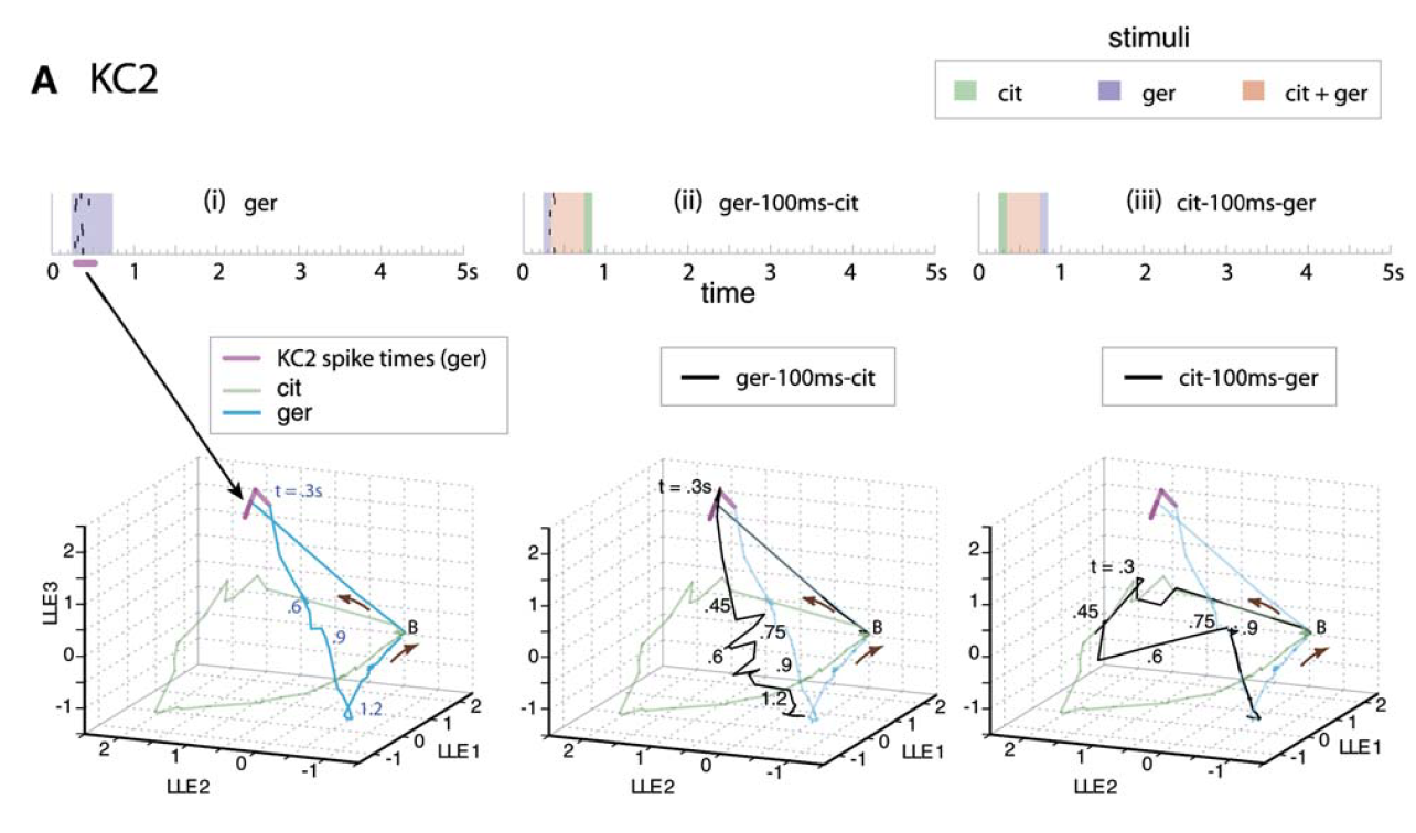
Spread of KC2 [Kenyon cell #2] spike times in response to geraniol (raster at top) overlaid (magenta) on PN ensemble responses as represented by LLE [locally linear embedding]. PN [antennal lobe projection neuron] ensemble responses are shown for the pure conditions (green, cyan) as well as two overlap conditions (black):
The firing times and strengths of KC2 are well matched to the instantaneous state of the PN trajectory.
Bede M. Broome et al. (2006). Encoding and Decoding of Overlapping Odor Sequences, Neuron 51:467-482.
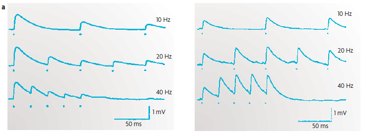
(a) An example of short-term plasticity of excitatory postsynaptic potentials (EPSPs) in excitatory synapses between [cortical] layer 5 pyramidal neurons. The traces represent the EPSPs from paired recordings; each presynaptic action potential is marked by a dot. Short-term plasticity can take the form of either short-term depression [contrast with LTD] (left) or short-term facilitation [contrast with LTP] (right).
The plots show that the strength of synapses can vary dramatically as a function of previous activity, and thus function as a short-lasting memory trace of the recent stimulus history.
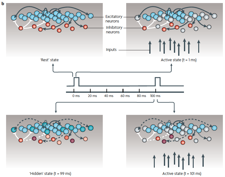
(b) Excitatory (blue) and inhibitory (red) neurons and some of their connections.
Top left: the baseline state, represented as quiescent (in reality there is spontaneous activity).
Top right: a brief stimulus generates action potentials in a subpopulation of the neurons (light gray shades).
Bottom left: "hidden" state. After the stimulus, as a result of short-term synaptic plasticity (dashed lines) and changes in intrinsic and synaptic currents (different color shades), the internal state may continue to change for hundreds of ms. Thus, although it is quiescent, the network should be in a different functional state at the time of the next stimulus (at t = 100ms).
Bottom right: because the network is in a different state, it would generate a different response pattern to the next stimulus, even if the stimulus is identical to the first one (a different pattern of blue spheres).
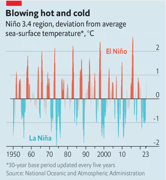
"El Niño and global warming are mixing in alarming ways. Havoc in poor countries and commodities markets is inevitable."
[From The Economist article, Aug 24th 2023]
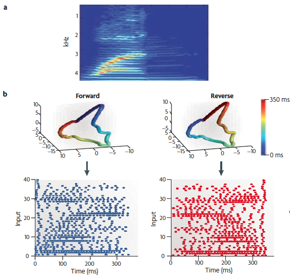
(a) A spectrogram of the spoken word "one".
(b) A cochlear model [here, a 40-neuron one] can be used to generate a spatiotemporal pattern of spikes generated by the word "one" (lower left). This pattern can be reversed (lower right) to ensure that the network is discriminating the spatiotemporal patterns of action potentials, as opposed to only the spatial structure. One can perform a principal-component analysis on the [binned averages of the] spikes of the input patterns, and by plotting the first three dimensions create a visual representation of the input trajectory. The upper panels show that the trajectories are identical except that they flow in opposite temporal directions. Time is represented in color: note the reverse color gradient.
Note that this signal from the cochlear model is just the input to the cortical model, illustrated on the next slide.
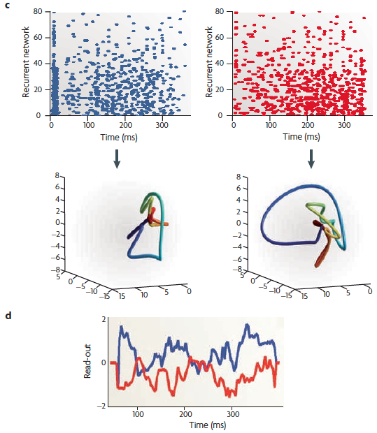
(c) The raster of an 80-neuron subset of a 280-neuron recurrent network in response to forward (blue) and reverse (red) directions. The neural trajectories (lower plots) show that the spatiotemporal spike patterns evoked by time-reversed stimuli are no longer the reverse of each other.
(d) A
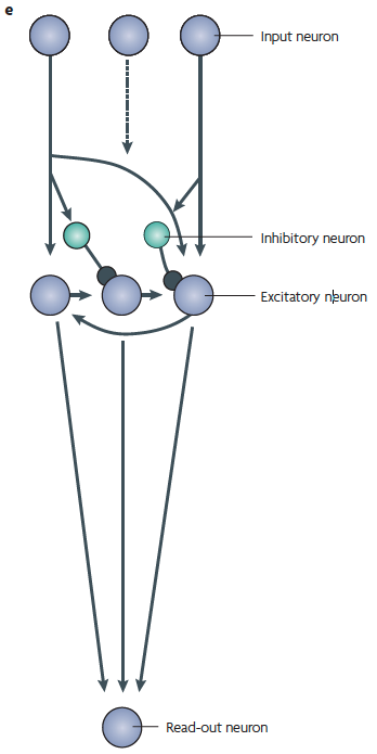
On the right — (e) A schematic of the [cortical microcircuitry model] recurrent network, with the components aligned with the relevant sections of parts (b)-(d). Several neurons provide input to excitatory neurons that are part of a recurrent network. The excitatory neurons in this network send a multi-dimensional signal to a single downstream read-out neuron.
On the left — pattern recognition in a bucket.
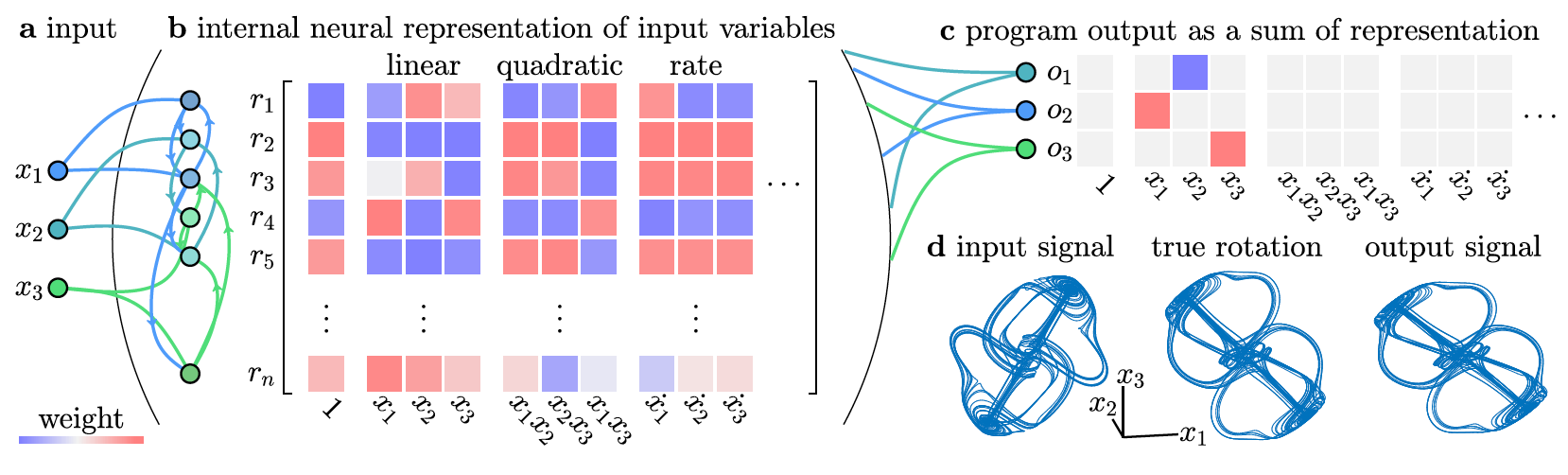
Unfurling neural states as a weighted sum of input variables.
A Neural Programming Language for the Reservoir Computer, Jason Z. Kim & Dani S. Bassett (2022). arXiv:2203.05032v1 [cond-mat.dis-nn].
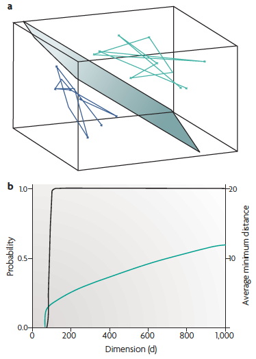
(a) Read-out can be computed as a linear combination (that is, weighted sum) \(w_1 x_1 + w_2 x_2 + \ldots w_d x_d\) of the inputs \(\textbf{x}\). Geometrically, the locus of points at which the weighted sum is exactly equal to a threshold is a hyperplane in the \(d\)-dimensional input space, illustrated here for \(d = 3\), together with two trajectories. Such perfect separation, however, cannot be expected in general.
(b) Mathematical results imply that
linear separation becomes much easier when the
dimension of the state space exceeds the "complexity" of the
trajectories. Black: the probability that 2 trajectories that
each linearly sequentially connect 100 randomly
chosen points can be separated by a hyperplane [the scale is on the
left vertical axis]. Green: the
average of the minimal Euclidean distance between pairs of
trajectories [right vertical axis]. In higher dimensions, not only
is it more likely that any two such trajectories can be separated,
but also they can be separated by a hyperplane with a larger
"safety margin".
Projections of external inputs into higher dimensions are quite common in the brain. For example, ~1 million axons from each optic nerve send visual information to the lateral geniculate nucleus, where it is combined with information from the pulvinar (another thalamic nucleus) and sent on to the primary visual cortex, in which there are ~500 million neurons.
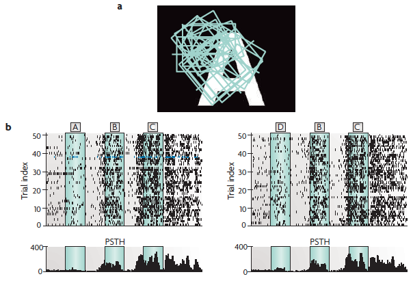
Population activity from the cat visual cortex encodes both the current and previous stimuli.
(a) A sample stimulus, with the receptive fields (squares) of the recorded neurons superimposed.
(b) The spike output of neuron number 10* for 50 trials with the letter sequence A, B, C as the stimulus and 50 trials with the letter sequence D, B, C as the stimulus. The temporal spacing and duration of each letter is indicated through green shading. The lower plot is a post-stimulus time histogram (PSTH) showing the response of neuron 10 over the 50 trials.
*Neuron 10 is shown in blue in part c on the next slide.
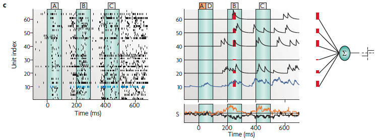
(c) The spike response of 64 neurons during trial number 38 for the letter sequence A, B, C (left; the blue trace shows the behavior of neuron 10 [from the previous slide]), and the read-out mechanism that was used to decode information from these 64 spike trains (upper right). Each spike train was low-pass filtered and sent to a linear discriminator.
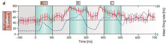
(d) The performance of a linear discriminator at various points in time. The red line shows the percentage of the cross-validated trials that the read-out correctly classified as to whether the first stimulus was A or D. The read-out neuron contained information about the first letter of the stimulus sequence even several hundred milliseconds after the first letter had been shown (and even after a second letter had been shown in the meantime). Note that discrimination is actually poor during the A and D presentation because of the low average firing rate (blue dashed lines).
[EXTRA: Are cats spying on us?]
[The
Quanta Magazine story.]
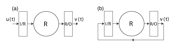
(a) Training data gathering phase. (b) Predicting phase.
It is assumed that the parameters of the reservoir are chosen such
that the “echo state property” is satisfied; i.e., all of the
conditional
Lyapunov exponents of the training reservoir
dynamics
conditioned on \({\bf u}(t)\) are negative so that, for large
\(t\), the reservoir state \({\bf r}(t)\) does not depend on
initial conditions.
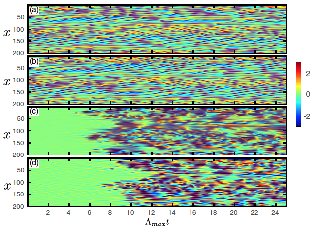
Prediction of KS equation \((L = 200, Q = 512, \mu = 0.01, \lambda = 100)\) with the parallelized reservoir prediction scheme using 64 reservoirs. (a) Actual KS equation data. (b) Reservoir prediction \([\tilde{{\bf u}}(t)]\). (c) Error in the reservoir prediction. (d) Error in a prediction made by integrating the KS equation when it uses the reservoir output at \(t = 0\), \([\tilde{{\bf u}}(0)]\), as its initial condition.
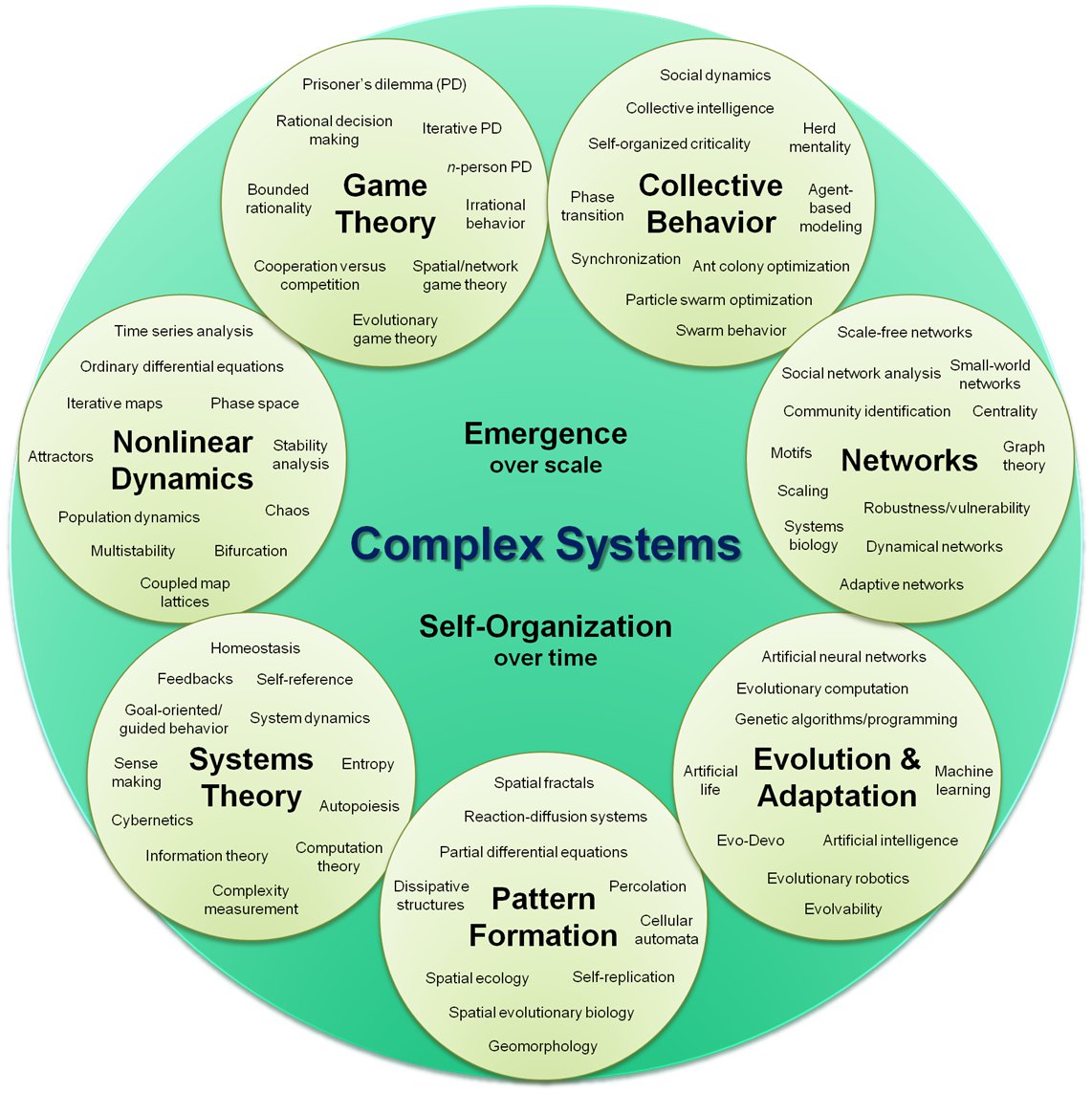
On the right: the subfields of the field of complex dynamical systems.
Why consider the DYNAMICS of the brain (as opposed to just the anatomy, or static snapshots of activity)???
A key concept is metastability, illustrated on slides 23 and 24.
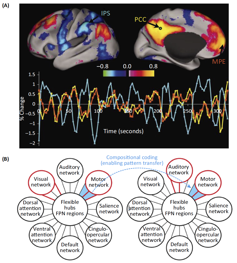
(A) Time series of anticorrelated switching in different FUNCTIONAL NETWORKS during resting state. Arrows indicate intraparietal sulcus (IPS), posterior cingulate/precuneus (PCC), and medial prefrontal cortex (MPF).
(B) Stimulus-dependent reorganization of the FUNCTIONAL CONNECTIVITY by the frontoparietal brain network (FPN) among visual, auditory, and motor systems across two different tasks. Global variable connectivity is depicted by the shifting connectivity pattern (red lines connecting FPN to other brain networks). The importance of sequential switching between network arrangements is signified by blue lines between the two networks.
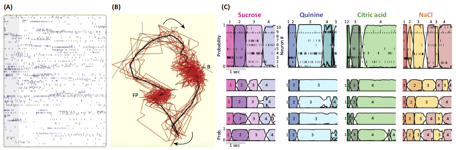
(A,B) the response to an odorant in an insect antennal lobe. It is the intrinsic transient dynamics of the complex antennal lobe system that maps such input to a sequential representation as seen in these single-trial responses of 110 antennal lobe neurons to one odor shown in (A) (gray bar, 1 s). Panel (B) shows the projections of neuron trajectories, representing the succession of states visited by this neural network in response to one odor. Red lines, individual trials; black line, average of ten trials. Abbreviations: B, baseline state; FP, fixed point, reached after 1.5 s.
(C) the taste-specific robust sequential pattern observed in neurons of the gustatory cortex of the rat in response to four taste stimuli. A model of joint temporal activity reveals that the network behavior is best represented by four discrete states in a WLC setting.
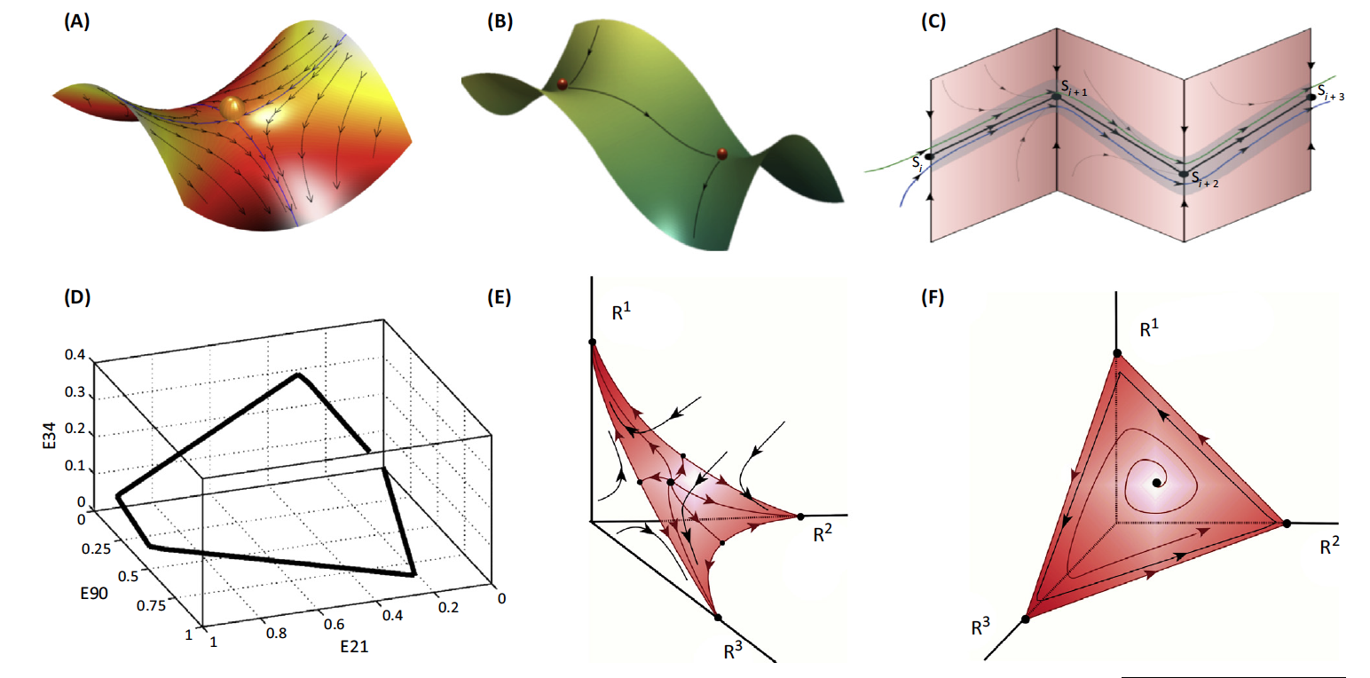
(A) A saddle with two stable and two unstable separatrices
(boundaries separating two modes of behavior). A set of saddles can
be sequentially connected by unstable separatrices (B) to form a
STABLE HETEROCLINIC CHANNEL (C).
(D) The low-dimensional heteroclinic dynamics of a large neuronal
model network – 200 excitatory/inhibitory neuronal clusters.
(E) The transient dynamics of attention; in this case, one
cognitive modality out of three requires full attention.
(F) Attention sharing (sequential switching of attention among
three different modalities) in the same model with different
intrinsic/extrinsic inputs.
Heteroclinic dynamics may serve an appropriate mathematical framework for robust transient processes that can be treated as an itinerary pass through metastable states. A heteroclinic channel is robust provided that the compression of the phase volume in the vicinity of the metastable states is stronger than the stretching, and trajectories that come to this area become prisoners, and thus unable to leave it.
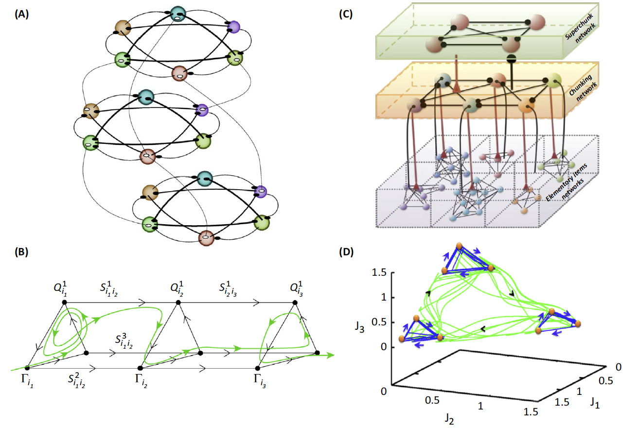
(A) An example of three modality binding networks in the context of
the discussed model (filled and unfilled circles: inhibitory and
excitatory connections).
(B) The corresponding phase
portrait of the binding dynamics. The
unstable separatrices that connect different metastable states are 2D in
this case. Q and \(\Gamma\): the metastable states; S are the corresponding
separatrices.
(C) An example of a three-level chunking hierarchical network
architecture. It can be, for example, text creation: with the first level
representing the organization of sentences; second level, paragraph
creation; and upper level, chapter organization. Spheres represent the
informational items or units (metastable states). Different colors
indicate different chunks. All connections inside the elementary items are
inhibitory.
(D) The corresponding phase portrait of the chunking activity in
the phase space of auxiliary variables. Blue trajectories represent the
dynamics inside the chunk. Green trajectories represent the chunk
sequential switching.