Unit 5: probability and the Bayes Theorem

getting to know the world; probability in cognition; the Bayes Theorem
- Getting to know the world
- The fundamental role of probability in cognition
- The Bayes Theorem [including a proof, which also appears in Appendix A in the book]
- Examples of the Bayes Theorem at work
the role of probability and statistics in cognition
How and in what sense can a cognitive system such as the brain get to KNOW
the world?
[Recall the war room analogy.]
Any system trying to get to know the world must deal with
UNCERTAINTY. Therefore, ...
the role of probability and statistics in cognition
How and in what sense can a cognitive system such as the brain get to KNOW
the world?
[Recall the war room analogy.]
Any system trying to get to know the world must deal with
UNCERTAINTY. Therefore, the following observation is crucially important:
"All knowledge resolves itself into probability"
David Hume
A Treatise of Human Nature (1740)
Probability theory is NOT about capitulating in
the face of uncertainty: it quantifies uncertainty and makes it formally
manageable.
on the importance of statistical data and methods

The joint probability distribution
$$
p(X,Y)
$$
is the most that can be known about
\(X\) and \(Y\) through observation.
[If you are allowed to intervene, you can
learn more, by doing science.]
You can estimate \(p(X,Y)\) by dividing the range of \(X\) and of \(Y\) into bins and
counting items that fall within each bin.
[Think of the values of \(X\) coding apple color; \(Y\) coding apple crunchiness.]
conditional probability, darts, and Venn diagrams
\(\require{color}\)

The
conditional probability of putting a
dart into that part of the inside of the big \(\textrm{O}\)
which is
\({\color{red} ♡}\)-colored
is defined as
$$
P(\textrm{O} \mid {\color{red} ♡}) = \frac{P(\textrm{O},{\color{red} ♡})}{P({\color{red} ♡})}
$$
-
Intuition: the conditional \(P(\textrm{O} \mid {\color{red} ♡})\)
is larger when the joint (intersection) \(P(\textrm{O},{\color{red}
♡})\) is larger; and smaller when the marginal \(P({\color{red}
♡})\) is larger (because then there are more ways of landing within
\({\color{red} ♡}\) but not within \(\textrm{O}\)).
-
An example: if you know how often apples are both OMGtasty and
\({\color{red} red}\),
\(P(OMGtasty,{\color{red} red})\), you can calculate the conditional probability of an apple
being OMGtasty, given that it is \({\color{red} red}\): by
definition,
$$
P(OMGtasty \mid {\color{red} red}) = \frac{P(OMGtasty,{\color{red}
red})}{P({\color{red} red})}
$$
using conditional probability in data-driven learning and generalization
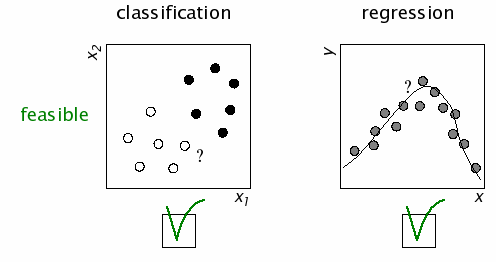
The computational essence of categorization and regression:*
Classification
1. estimate the probability of each possible class label, given the values
of the object's features:
$$
p({\cal C}_i \mid x_1, x_2)
$$
2. choose
the class with the largest probability.
Example: categorization (given \(size\) and \(color\), predict \(crunchy/mushy\)).
Regression
1. estimate the probability of each possible output value,
given the input value(s):
$$
p(y \mid x)
$$
2. choose the output value
with the largest probability.
Example: estimation (given \(color\), predict \(HOW tasty\)); also
visual-motor coordination.
*
NOTE: input/output or I/O mapping (which includes categorization and regression)
by no means covers everything that minds do to control behavior,
but it is an indispensable conceptual starting point.
conditional probability and the view of generalization as statistical inference
The computational essence of categorization and regression:
— Both classification and regression are underdetermined and
therefore must rely on extra assumptions (as in regularization; more about this next week).
— Both reduce to
probability estimation.
the kind of probability estimation required for learning and generalization
Continuing the example of learning to deal with apples:
\({\cal C}_1\) = "crunchy apple"
\({\cal C}_2\) = "mushy apple"
\(x_1\) : color dimension
\(x_2\) : size dimension
There is a bit of a problem.
Suppose that we're looking at an apple \(A\)
that has color \(x_1^{(A)}\) and size \(x_2^{(A)}\).
| from experience, we may know |
\(p\left(x_1^{(Z)}, x_2^{(Z)} \mid {\cal C}_1\right)\) |
— how often the crunchy apples \(Z\) we tasted happened to be of
a particular color and size |
| but what we need to know is |
\(p\left({\cal C}_1 \mid x_1^{(A)}, x_2^{(A)}\right)\) |
— how likely an apple \(A\) of this color and
size is to be crunchy (before tasting it) |
the kind of probability estimation required for learning
HELP!!!
is on the way: the Bayes Theorem.
the Bayes Theorem follows immediately from the definition of conditional probability
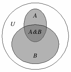
The
conditional probability of
B given
A
(think darts) is defined as the ratio of two areas:
$$
p(B \mid A) = \left\vert A \& B\right\vert / \left\vert A\right\vert
$$
On the right, divide numerator and denominator by the area of the
"universe" \(\left\vert U\right\vert\) to obtain a ratio of probabilities:
$$
p(B \mid A) = p(A \& B) / p(A)
$$
Now, by the definition of
conditional probability,
the
joint probability, which depends symmetrically on \(A\)
and \(B\), can be expressed in two equivalent ways:
$$
\begin{align}
p(A \& B) &= p(A) p(B \mid A) = \\
&= p(B) p(A \mid B) = p(B \& A)
\end{align}
$$
Suppose
\(B\) is a hypothesis ("apple is
crunchy"), and
\(A\)
is data ("apple is red"). We can now
estimate the
probability of the
hypothesis being true, given the
data:
$$
p({\color{gray} B} \mid \mathbf{A}) = \frac{p(\mathbf{A} \mid
{\color{gray} B}) p({\color{gray} B})}{p(\mathbf{A})}
$$
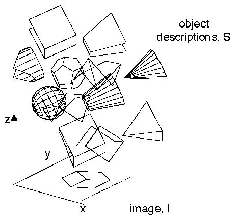
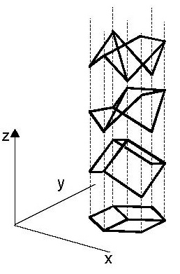
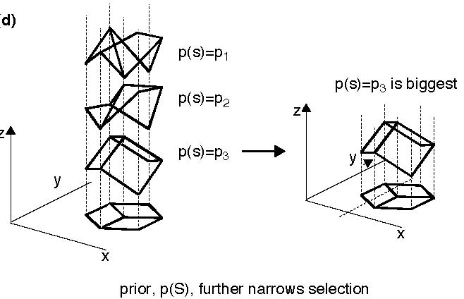
an application: Bayes in wireframe shape perception
 |
 |
|
Must find the probabilities of various conceivable shape
interpretations (hypotheses),
given the image (data). According to Bayes, $$p(S\mid I) \propto p(I\mid S)p(S)$$
|
The likelihood term, \(p(I\mid S)\), rules out shapes \(S\)
that are inconsistent with the image \(I\) (here, spheres,
cones, etc.).
|
Bayes in wireframe shape perception (cont.)
the big picture: the probabilistic approach to cognition (Chater et al., 2006)
"The brain is an information processor; and information processing
typically involves inferring new information from information that has
been derived from the senses, from linguistic input, or from memory. This
process of inference from old to new is, outside pure mathematics,
typically uncertain."
"Probability theory is, in essence, a calculus for uncertain inference,
according to the SUBJECTIVE INTERPRETATION OF PROBABILITY.
Thus probabilistic methods have potentially broad application
to uncertain inferences:
— from sensory input to environmental layout;
— from speech signal to semantic interpretation;
— from goals to motor output;
— or from observations and experiments to regularities in nature."
subjective probability (Chater et al., 2006)
"Crucially, the frequency interpretation of probability is not in play
here — in cognitive science applications, probabilities refer to 'DEGREES
OF BELIEF'.
Thus, a person's degree of belief that a coin that has rolled
under the table has come up heads might be around 1/2; this degree of
belief might well increase rapidly to 1 as she moves her head, bringing
the coin into view. Her friend, observing the same event, might have
different prior assumptions and obtain a different stream of sensory
evidence.
Thus the two people are viewing the same event, but their belief
states and hence their subjective probabilities might differ. Moreover,
the relevant information is defined by the specific details of the
situation. This particular pattern of prior information and evidence will
never be repeated, and hence cannot define a limiting frequency."
working with subjective probabilities (Chater et al., 2006)
The centrality of Bayes' Theorem to the subjective approach to
probability has led to the approach commonly being known as the
Bayesian approach. But the real content of the approach is the
subjective interpretation of probability; Bayes' Theorem
itself is just an elementary, if spectacularly productive,
identity in probability theory."
[The following is a paraphrase of what has been stated on
previous slides.]
"The subjective interpretation of probability generally aims to
evaluate CONDITIONAL PROBABILITIES, \(Pr(h_j\mid d)\), that is,
probabilities of alternative hypotheses, \(h_j\) (about the
state of reality), given certain data, \(d\) (e.g. available to
the senses). By the definition of conditional probability, for
any propositions, \(A\) and \(B\), the probability that both are
true, \(Pr(A, B)\), is by definition the probability that \(A\)
is true, \(Pr(A)\) , multiplied by the probability that \(B\) is
true, given that \(A\) is true, \(Pr(B\mid A)\) .
Applying this identity, simple algebra [see slide 12] gives Bayes' Theorem:
$$
Pr(h_j \mid d) = \frac{Pr(d \mid h_j) Pr(h_j)}{Pr(d)}
$$
probability models are useful on many levels (Chater et al., 2006)
"Sophisticated probabilistic models can be related to cognitive processes
in a variety of ways. This variety can usefully be understood in terms of
Marr's celebrated distinction between three levels of computational
explanation: the computational level, which specifies the nature of the
cognitive problem being solved, the information involved in solving it,
and the logic by which it can be solved; the algorithmic level, which
specifies the representations and processes by which solutions to the
problem are computed; and the implementational level, which specifies how
these representations and processes are realized in neural terms.
Finally, turning to the implementational level, one may
ask whether THE BRAIN ITSELF SHOULD BE VIEWED IN PROBABILISTIC
TERMS. Intriguingly, many of the sophisticated probabilistic models that
have been developed with cognitive processes in mind map naturally onto
highly distributed, autonomous, and parallel computational architectures,
which seem to capture the qualitative features of neural
architecture."
basic Bayes: how to use the estimated posterior? (Griffiths & Yuille, 2006)
Assume that we have an agent who is attempting to infer the process that
was responsible for generating some data, \(d\). Let \(h\) be a hypothesis about
this process, and \(P(h)\) — the prior probability that the agent would have
accepted \(h\) before seeing \(d\). How should the agent's beliefs change
in the light of the evidence provided by \(d\)? To answer this question, we
need a procedure for computing the posterior probability, \(P(h
\mid d)\). This is provided by the Bayes Theorem:
$$
P(h \mid d) = \frac{P(d \mid h) P(h)}{P(d)}
$$
How can the posterior be used to guide action?
The denominator is obtained by summing over [the mutually exclusive]
hypotheses, a procedure known as marginalization:
$$
P(d) = \sum_{h^{\prime}\in H} P(d \mid h^{\prime}) P(h^{\prime})
$$
where \(H\) is the set of all hypotheses considered by the agent.
using the posterior: Bayesian decision & control (Griffiths & Yuille, 2006, Box 1)
Bayesian decision theory introduces a loss function \(L\left(h,
\alpha\left(d\right)\right)\) for the cost of making a decision \(\alpha(d)\) when the
input is \(d\) and the true hypothesis [true state of affairs] is \(h\). It proposes selecting the
decision function or rule \(\alpha^{\star}(\cdot)\) that minimizes the RISK, or
EXPECTED LOSS:
$$
R(\alpha) = \sum_{h,d} L\left(h, \alpha\left(d\right)\right) P(h, d)
$$
This is the basis for RATIONAL DECISION MAKING.
In classification, \(L\) can be chosen so that the same penalty is paid for all
wrong decisions:
\(L\left(h, \alpha\left(d\right)\right) = 1\) if \(\alpha\left(d\right) \neq h\)
and
\(L\left(h, \alpha\left(d\right)\right) = 0\) if \(\alpha\left(d\right) = h\).
Then the best decision rule
is the maximum a posteriori (MAP) estimator
\(\alpha^{\star}(d) = \textrm{argmax}_{h} P(h \mid d)\).
using the posterior: Bayesian decision & control (Griffiths & Yuille, 2006, Box 1)
Bayesian decision theory introduces a loss function \(L\left(h,
\alpha\left(d\right)\right)\) for the cost of making a decision \(\alpha(d)\) when the
input is \(d\) and the true hypothesis [true state of affairs] is \(h\). It proposes selecting the
decision function or rule \(\alpha^{\star}(\cdot)\) that minimizes the RISK, or
EXPECTED LOSS:
$$
R(\alpha) = \sum_{h,d} L\left(h, \alpha\left(d\right)\right) P(h, d)
$$
This is the basis for RATIONAL DECISION MAKING.
In regression, the loss function can take the form of the square of the error:
\(L\left(h, \alpha\left(d\right)\right) = \left\{h−\alpha\left(d\right)\right\}^2\)
Then the best solution is the
posterior mean, that is, the probabilistically weighted average
of all possible (numerical in this case) hypotheses: \(\sum_{h} h P(h \mid d)\).
[EXTRA] generative vs. empirical risk minimization approaches
An important distinction: generative models vs. empirical risk minimization approaches —
In many situations, we will not know the distribution \(P(h, d)\) exactly
but will instead have a set of labelled samples \(\left\{\left(h_i, d_i\right) : i =
1,\dots,N\right\}\). The risk
$$
R(\alpha) = \sum_{h,d} L\left(h, \alpha\left(d\right)\right) P(h, d)
$$
can then be approximated by the empirical
risk,
$$
R_{emp}(\alpha) = \frac{1}{N} \sum_{i=1}^{N} L\left(h_i, \alpha\left(d_i\right)\right)
$$
Some methods used in machine learning, such as certain "neural networks" and support
vector machines, attempt to learn the decision rule directly by minimizing
\(R_{emp}(\alpha)\) instead of trying to model \(P(h, d)\).
More importantly for us, BRAINS may have evolved to apply either or
both of these two approaches in the context of a particular class of
tasks. The distinction between them is similar to the one between
"model-based" and "model-free" reinforcement learning, which I'll
discuss in Unit 9.


