reinforcement learning in motor and other tasks

• A closer look at motor learning
• Classes of control
• From error-based to reinforcement learning
• Representations in reinforcement learning. The Credit Assignment Problem
• Hierarchical RL

levels of understanding of motor learning (after Wolpert, 2011)

• The task components that must be learned for skilled performance, including:
  • efficient gathering of task-relevant sensory information;
  • selection strategy;
  • decision making;
  • balancing predictive and reactive control.
• The learning processes that apply to these components:
  • how errors and rewards drive learning;
  • what are the representations involved and how they are modified;
  • how credit is assigned and how learning generalizes to novel situations.
• the neural mechanisms of motor learning and memory, including:
  • the circuits involved;
  • synaptic modification.

classes of control

In general, optimizing motor performance is achieved through three classes of control:

• predictive or feedforward control, which is critical given the feedback delays in the sensorimotor system;
• reactive or feedback control, which involves the use of sensory inputs to update ongoing motor commands; and
• biomechanical control, which involves modulating the compliance of the limb.

---

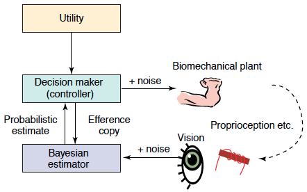
[EXTRA] The Bayesian framework has many uses in sensorimotor learning. Sensory integration. Multiple streams of sensory information, within and across modalities (for example, visual and tactile inputs), can be optimally combined to achieve estimates that reduce the effects of noise. This integration process can take into account the properties of external objects, such as tools, so that the visuo-haptic integration is optimal even when the tactile input comes through a hand-held tool. Learning priors. By learning the statistical distribution of possible states of the world, the estimate can be further refined. Developing and using internal models. By combining these processes with internal models of the body that map the motor commands (as signalled through the efference copy) into the expected sensory inputs, Bayesian inference can be used to estimate the evolving state of our body and the world.

learning from one's errors

Error-based learning is the key process in many well-studied ADAPTATION paradigms, including

• prism adaptation,
• saccade adaptation,
• reaching in force fields,
• visuomotor adaptation,
• grip force adaptation.

A common feature across these different task domains:

The system can — and will — learn from an error in a single trial.
Thus, adaptation is observable even when all perturbations are random (that is, unexpected) and the subject is told not to adapt.

from error-based to reinforcement learning

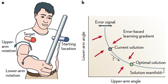
(a) A simple redundant task in which a target has to be reached with a stick using two effectors: shoulder and arm, whose rotations together contribute to a combined outcome.
(b) Many combinations of the two rotations will on average produce the correct solution. The locus of these is the solution manifold; the error signal corresponds to deviations from it (blue double arrow).

• For error-based learning to occur, the system needs to apportion the error to each of the two effectors, by following the error-based learning gradient (red arrows).
• However, to find a less variable or less effortful 'optimal' solution (green circle) along the solution manifold (direction shown by a dashed arrow), other learning mechanisms, such as reinforcement learning (RL), are needed.

In contrast to an error signal, reinforcement signals — which can be as simple as "success" or "failure" — do not give information about the required control change. Thus, the learner must explore the possibilities to gradually improve its motor commands. Like error-based learning, RL can also be used to guide learning towards the solution manifold. However, because the signal (the reward) provides less information than in error-based learning (the vector of errors), such learning tends to be SLOW.

representations (models) in reinforcement learning

Information obtained during a single movement is often too sparse or too noisy to unambiguously determine the source of the error. Therefore, it underspecifies the way in which the motor commands should be updated, resulting in an inverse problem (differences in control uniquely specify differences in outcome, but not vice versa).

To resolve this issue, the system does not start from a blank slate. Instead, it uses models of the task: representations that reflect its assumptions about the task structure and that constrain error-driven learning. Such models can be mechanistic or normative.

Mechanistic models specify the representations and learning algorithms directly. In this framework, representations are often considered to be based on motor primitives (the neural building blocks out of which new motor memories are formed; cf. synergies illustrated in slides 9—11).

Normative models specify optimal ways for the learner to adapt when faced with errors. A normative model includes two key components:

1. a GENERATIVE MODEL of the situation, which specifies how different factors, such as tools or levels of fatigue, influence performance;
2. a prior distribution, which states how these factors are likely to vary over space and time.

mechanistic models: motor primitives and structural learning

Motor primitives can be thought of as neural control modules that can be flexibly combined to generate a large repertoire of behaviors. For example, a primitive might represent the temporal profile of a particular muscle activity. The overall motor output will be could be the sum of all primitives, weighted by the level of the activation of each module. The makeup of the population of such primitives then determines which structural constraints are imposed on learning.

Several recent models have been developed to account for the reduction in interference in the presence of contextual cues. These models propose multiple, overlapping internal representations that can be selectively engaged by each movement context.

A general underlying principle of what can or cannot serve as a contextual switch has NOT been identified.

[Compare the Frame Problem that arises in connection with knowledge representation and truth maintenance.]

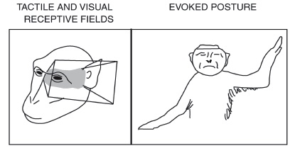
motor primitives: synergies in monkey motor cortex

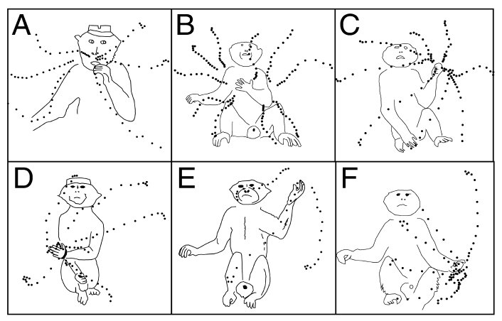
Motor control is HIERARCHICAL: some of the primitives (units) of action that it involves are very high-level.

The illustration shows the postural MOVEMENT SYNERGIES evoked by stimulating single neurons in monkey precentral gyrus (from Graziano et al., 2002).

synergies in ant motor control

The zombie ant phenomenon shows what happens when motor/action synergies are hijacked.

postural synergies (from Graziano et al., 2002)

Defense postures in monkey, man, and woman (the painting is a detail from Michelangelo's Fall and Expulsion from Eden).

normative models: the credit assignment problem

Within the normative framework, the process of motor [or any other kind of] learning can be understood as a credit assignment problem (see Marvin Minsky's 1960 paper where it is first stated): how to attribute an error signal to the underlying causes.

For example, if a tennis player starts hitting shots into the net on the serve, the problem could be that the ball was not thrown high enough, was hit too early, that the racquet strings are loose or that he or she is fatigued. If the racquet dynamics have changed, the player would do well to learn these dynamics and remember them for the next time that they use this particular racquet. Conversely, if the player is simply tired, the necessary adjustments should only be temporary but should be applied even if the racquet is changed at that moment.

Two types of credit assignment can be distinguished:

• contextual/structural;
• temporal.

from motor control to general decision-making (Dayan & Niv, 2008)

Like motor control, general decision making environments are characterized by:

• a STATE SPACE (states are such things as locations in a maze or board positions in a game);
• a set of actions (directions of travel, moves on a board);
• affectively important outcomes (finding cheese, obtaining water, winning).

Actions can move the decision-maker from one state to another and they can produce outcomes.

The outcomes are assumed to have numerical (positive or negative) UTILITIES, which can change according to the motivational state of the decision-maker (e.g. food is less valuable to a satiated animal).

Typically, the decision-maker starts off not knowing the rules of the environment (the state transitions and outcomes brought about by the actions), and has to learn or sample these from experience.

an example of a STATE SPACE: the Towers of Hanoi problem

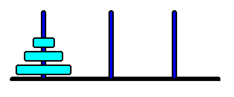
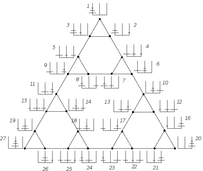
The 3-disk version of the Towers of Hanoi problem...	...and its STATE SPACE.

model-free compared to model-based RL (Dayan & Niv, 2008)

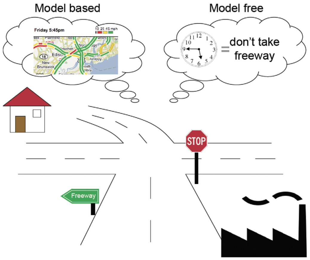Right: an illustration of the difference between model-free and model-based approaches to decision-making.

---

Model-free vs. model-based RL, from Theoretical Impediments to Machine Learning With Seven Sparks from the Causal Revolution (2018) by the great Judea Pearl:

"The philosopher Stephen Toulmin (1961) identifies model-based vs. model-blind dichotomy as the key to understanding the ancient rivalry between Babylonian and Greek science. According to Toulmin, the Babylonians astronomers were masters of black-box prediction, far surpassing their Greek rivals in accuracy and consistency (Toulmin, 1961, pp. 27–30). Yet Science favored the creative-speculative strategy of the Greek astronomers which was wild with metaphysical imagery: circular tubes full of fire, small holes through which celestial fire was visible as stars, and hemispherical earth riding on turtle backs. Yet it was this wild modeling strategy, not Babylonian rigidity, that jolted Eratosthenes (276-194 BC) to perform one of the most creative experiments in the ancient world and measure the radius of the earth. This would never have occurred to a Babylonian curve-fitter."

types of operant learning (Shteingart & Loewenstein, 2014)

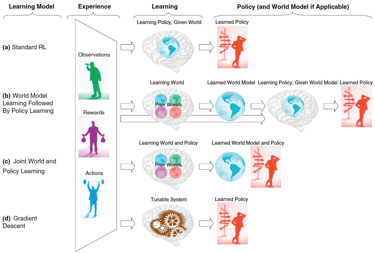
In operant learning, experience (left trapezoid), composed of present and past observations, actions and rewards, is used to learn a "policy".

(a) Standard RL models typically assume that the learner (brain gray icon) has access to the relevant states and actions set (represented by a bluish world icon) before the learning of the policy. Alternative suggestions are that the state and action sets are learned from experience and from prior expectations (different world icons) before (b) or in parallel (c) to the learning of the policy. (d) Alternatively, the agent may directly learn without an explicit representation of states and actions, but rather by tuning a parametric policy (cog wheels icon), for example, using stochastic gradient methods on this policy’s parameters.

reinforcement learning: the MDP formulation and link to algorithms

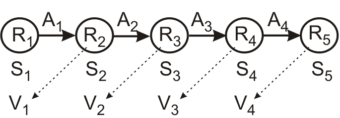
The best studied case is when RL can be formulated as a class of Markov Decision Problems (MDP).

The agent can visit a finite number of states \(S_i\). In visiting a state, it collects a numerical reward \(R_i\), where negative numbers may represent punishments. Each state has a changeable value \(V_i\) attached to it. From every state there are subsequent states that can be reached by means of actions \(A_{ij}\). The value \(V_i\) of a state \(S_i\) is defined by the averaged future reward \(\tilde{R}\) which can be accumulated by selecting actions from this particular state. Actions are selected according to a policy which can also change. The goal of an RL algorithm is to select actions that maximize the expected cumulative reward (the return) of the agent.

[For a useful introduction to RL, MDP, and the basic algorithms, see the Scholarpedia article.]

the agent, the environment, and the nature of reward (Barto, 2013)

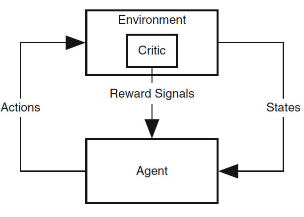
The old/standard view of agent-environment interaction in RL. Primary reward signals are supplied to the agent from a "critic" in its environment.

---

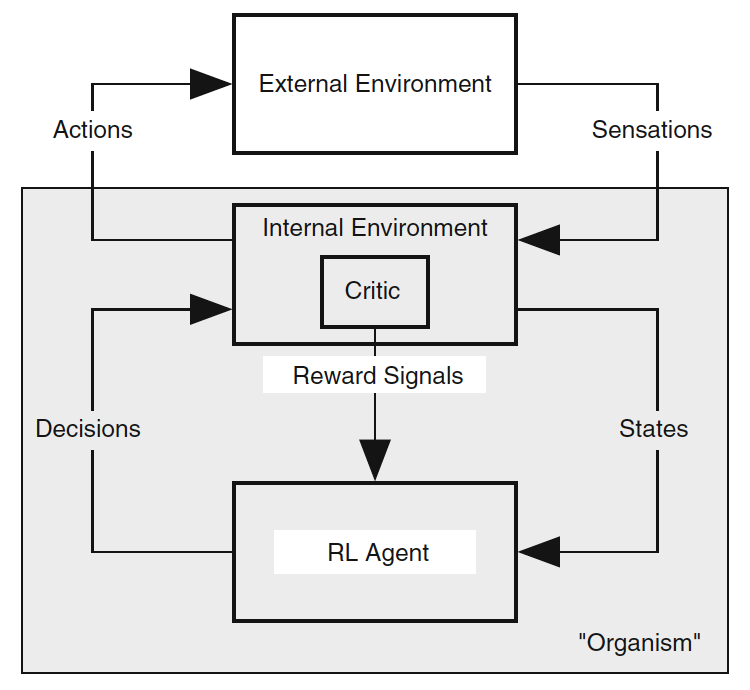
A refined view, in which the environment is divided into an internal and external environment, with all reward signals coming from the former. The shaded box corresponds to what we would think of as the "organism."

---

With this insight into the nature of the reward, the proper approach to RL is intrinsically motivated reinforcement learning.

HIERARCHICAL [model-free] reinforcement learning

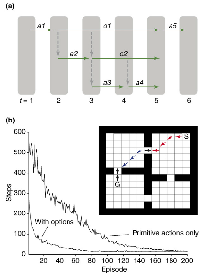
(a) A schematic of action selection in the OPTIONS framework. At the first time-step, a primitive action, a1, is selected. At time-step two, an option, o1, is selected, and the policy of this option leads to selection of a primitive action, a2, followed by selection of another option, o2. The policy for o2, in turn, selects primitive actions a3 and a4. The options then terminate, and another primitive action, a5, is selected at the top-most level.

(b) Inset: the rooms domain (Sutton et al.), as implemented by Botvinick et al.

S, start; G, goal. Primitive actions include single-step moves in the eight cardinal directions. Options contain policies to reach each door. Arrows show a sample trajectory involving selection of two options (red and blue arrows) and three primitive actions (black). The plot shows the mean number of steps required to reach the goal over learning episodes with and without inclusion of the door options.

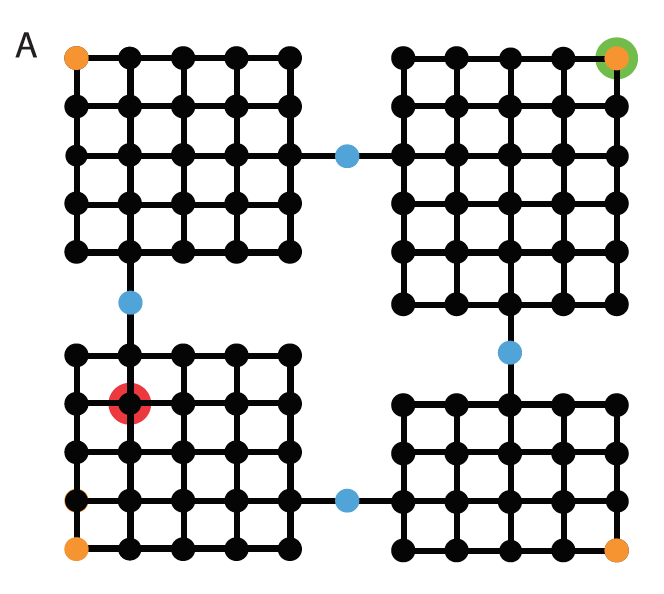
HIERARCHICAL [model-based] reinforcement learning

Looking for optimal task hierarchy:

"Arranging actions hierarchically has well established benefits, allowing behaviors to be represented efficiently by the brain, and allowing solutions to new tasks to be discovered easily. However, these payoffs depend on the particular way in which actions are organized into a hierarchy, the specific way in which tasks are carved up into subtasks. We provide a mathematical account for what makes some hierarchies better than others, an account that allows an optimal hierarchy to be identified for any set of tasks. We then present results from four behavioral experiments, suggesting that human learners spontaneously discover optimal action hierarchies."

— Optimal Behavioral Hierarchy (2014), by Alec Solway, Carlos Diuk, Natalia Córdova, Debbie Yee, Andrew G. Barto, Yael Niv, and Matthew M. Botvinick.

---

(A). Rooms domain. Vertices represent states (green = start, red = goal), and edges feasible transitions.

[EXTRA] optimal behavioral hierarchy (Solway et al. 2014)

"The optimal hierarchy is one that best facilitates adaptive behavior in the face of new problems. [...] This notion can be made precise using the framework of Bayesian model selection. [...] The agent is assumed to occupy a world in which it will be faced with a specific set of tasks in an unpredictable order, and the objective is to find a hierarchical representation that will beget the best performance on average across this set of tasks. An important aspect of this scenario is that the agent may reuse subtask policies across tasks (as well as task policies if tasks recur)."

In Bayesian model selection, each candidate model is assumed to be associated with a set of parameters \(\theta\), and the fit between the model and the target data is quantified by the marginal likelihood or model evidence: $$ Pr(data\vert model)=\sum_{\theta\in\Theta} Pr(data\vert model,\theta) Pr(\theta\vert model) $$ where \(\Theta\) is the set of feasible model parameterizations (in the above formula, the likelihood is called "marginal" because it is marginalized over all possible choices of \(\theta\)).

[EXTRA] optimal behavioral hierarchy (Solway et al. 2014)

In the present setting, where the models in question are different possible hierarchies, and the data are a set of target behaviors, the model evidence becomes: $$ Pr(behavior\vert hierarchy)=\sum_{\pi\in\Pi} Pr(behavior\vert hierarchy,\pi) Pr(\pi\vert hierarchy) $$ where \(\Pi\) is the set of behavioral policies \(\pi\) available to the candidate agent, given its inventory of subtask representations (this includes the root policy for each task in the target ensemble, as well as the policy for each subtask itself).

---

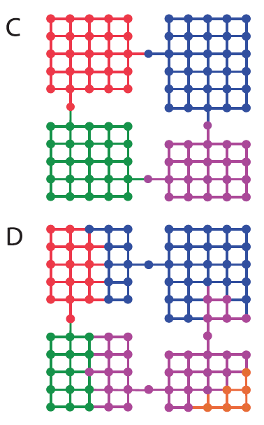
(C). Optimal decomposition. (D). An alternative decomposition.

[EXTRA] optimal behavioral hierarchy (Solway et al. 2014)

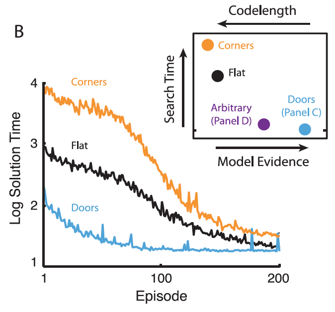
(B). Mean performance of three hierarchical reinforcement learning agents in the rooms task.

Inset: Results based on four graph decompositions. Blue: decomposition from panel C [previous slide]. Purple: decomposition from panel D. Black: entire graph treated as one region. Orange: decomposition with orange vertices in panel A segregated out as singleton regions.

Model evidence is on a log scale (data range \( -7.00 \times 10^4\) to \( -1.19 \times 10^5\)). Search time denotes the expected number of trial-and-error attempts to discover the solution to a randomly drawn task or subtask (geometric mean; range 685 to 65947; tick mark indicates the origin). Codelength signifies the number of bits required to encode the entire data-set under a Shannon code (range \(1.01\times 10^5\) to \(1.72\times 10^5\)). Note that the abscissa refers both to model evidence and codelength. Model evidence increases left to right, and codelength increases right to left.

[EXTRA] optimal behavioral hierarchy (Solway et al. 2014)

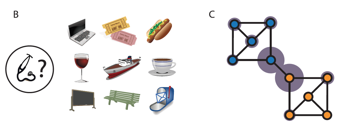
(B). Task display from Experiment 1. Participants used the computer mouse to select three locations adjacent to the probe location.

(C). Graph employed in Experiment 1, showing the optimal decomposition. Width of each gray ring indicates mean proportion of cases in which the relevant [bus stop^*] location was chosen.

---

^* Following this training period, participants were informed that they would next be asked to navigate through the town in order to make a series of deliveries between randomly selected locations, receiving a payment for each delivery that rewarded use of the fewest possible steps. Before making any deliveries, however, participants were asked to choose the position for a ‘‘bus stop’’ within the town. Instructions indicated that, during the subsequent deliveries, participants would be able to ‘‘take a ride’’ to the bus stop’s location from anywhere in the town, potentially saving steps and thereby increasing payments. Participants were asked to identify three locations as their first-, second- and third-choice busstop sites.

[EXTRA] optimal behavioral hierarchy (Solway et al. 2014)

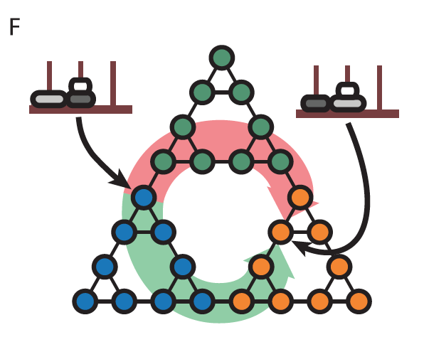
(F). State-transition graph for the Tower of Hanoi puzzle, showing the optimal decomposition and indicating the start and goal configurations of the kind studied in Experiment 4.