Lecture 12.1: learning via synaptic modification

• computational models of synaptic learning:
  • the Hebb rule and the Oja rule
  • the BCM rule / projection pursuit
• biological relevance of the BCM rule

a by-now-unnecessary reminder: how a neuron computes

The basic computation performed by a neuron:

1. multiply the components of the incoming signal \(\textbf{x}=(x_1,x_2,\dots,x_i)\) by their corresponding synaptic weights, \(\textbf{w}=(w_1,w_2,\dots,w_i)\)
2. sum the resulting products;
3. pass the sum through a nonlinearity (e.g., logistic sigmoid);
4. compare the result to a threshold;
5. if it exceeds the threshold, then output an action potential (spike).

how neurons learn: experience driving the changes

In many types of neurons, the synaptic weight \(\textbf{w}\) is modifiable by experience (and so are some of the parameters that control this modification process; see slides #10-#11).

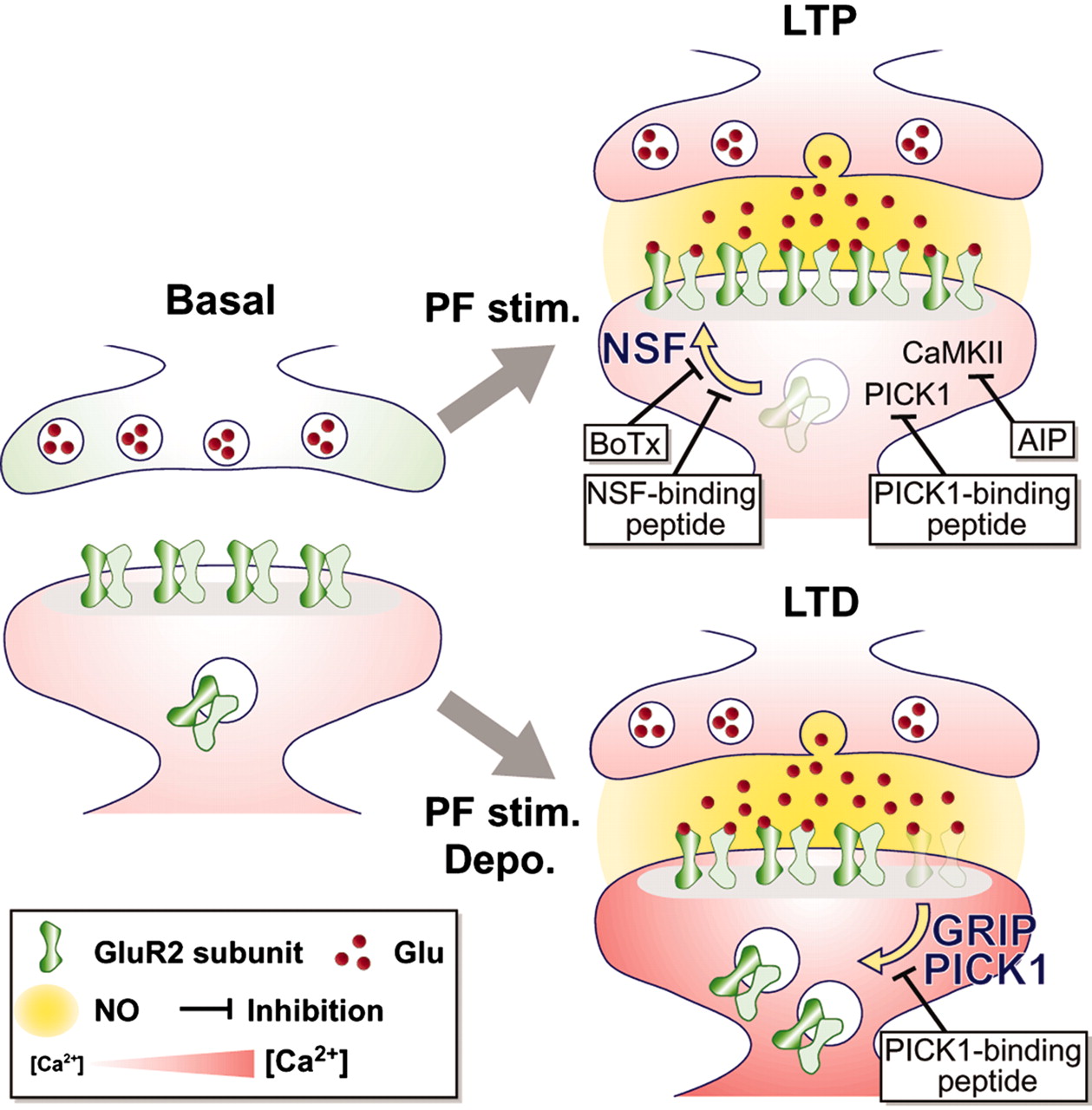
Synaptic modification can take the form of Long-Term Potentiation (LTP) or Long-Term Depression (LTD) of synaptic efficacy (weight).

The details of these processes — even the vastly oversimplified sketch of the molecular dynamics of LTP and LTD illustrated here — are beyond the scope of the present discussion.

Experience = joint statistics of presynaptic and postsynaptic neuron activities.

a reminder re the neuron's "experience": the War Room analogy

Experience = joint statistics of presynaptic and postsynaptic neuron activities.

Why it makes sense to define experience in terms of SYNAPSE-level events:

Why it makes sense to consider experience through the lens of STATISTICS:

Why JOINT INPUT&OUTPUT statistics?

[to keep in mind: types of learning]

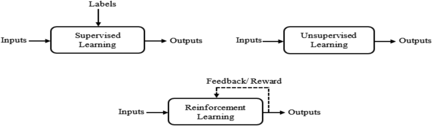
What types of learning best describe which NATIVE computations in biological nervous systems?

What about neural computations carried out in VIRTUAL mode?

ONE RULE TO BRING THEM ALL

The Mordor rule:

The Hebbian rule:

[That's just the short of it. There's A LOT of nuance.]

input space and weight space, visualized together

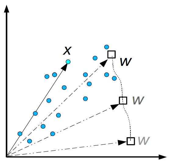
Consider a neuron with two inputs that computes $$ y = \textbf{w}\cdot \textbf{x} = w_1 x_1 + w_2 x_2 $$

On the right, the input \(\textbf{x}=(x_1,x_2)\) and the weight \(\textbf{w}=(w_1,w_2)\) vectors are plotted together in the same 2D space. The dotted line shows the change that the weight vector undergoes through Hebbian learning (see next slide).

In the plot here, the horizontal and vertical axes are for \((x_1,x_2)\), which is the input space, and for \((w_1,w_2)\), which is the weight space.

input/output statistics driving weight changes

Consider a neuron that computes $$ y = \textbf{w}\cdot \textbf{x} = w_1 x_1 + w_2 x_2 $$

Computational analysis carried out in the 1980s^* showed that a neuron with experience-dependent Hebbian synapses (as in: spike timing dependent plasticity, STDP, to be discussed later this week) learns the projection [of the input vector onto its weight vector] that maximizes the variance of the data in the resulting output space. In other words, it carries out Principal Component Analysis or PCA.

In the plot here, the horizontal and vertical axes are for \((x_1,x_2)\) and \((w_1,w_2)\).

^* Sanger, T. D. (1989). Optimal unsupervised learning in a single-layer linear feedforward neural network. Neural Networks 2:459-473.

the Hebb rule and Oja's modification of it

Hebbian learning: a synaptic connection between two neurons increases in efficacy in proportion to the degree of correlation between the mean activities of the pre- and post-synaptic neurons (Donald O. Hebb, 1949).

The Hebb rule in formal notation: the rate of change (time derivative) of the weight \(w_i\) is proportional to the product of the input \(x_i\) and output \(y\) — $$ \begin{matrix} y &=& \sum_i w_i x_i \\ \frac{dw_i}{dt} &=& \eta x_i y \end{matrix} $$ The Oja rule: $$ \frac{dw_i}{dt} = \eta \left(x_i y - y^2w_i\right) $$

an axiomatic approach to modeling synaptic modification, leading to the BCM rule (after Cooper & Bear 2012)

To account for much data on synapse modification in response to experience, Bienenstock, Cooper, and Munro (1982) proposed the three postulates of what came to be called the BCM theory:

1. The change in synaptic weights (\(dw_i/dt\)) is proportional to the PREsynaptic activity (\(x_i\)).
2. The change in synaptic weights (\(dw_i/dt\)) is also proportional to a non-monotonic function (denoted by \(\phi\)) of the POSTsynaptic activity (\(y\)), such that:
   1. for small \(y\) , the synaptic weight decreases (\(dw_i/dt < 0\));
   2. for larger \(y\) , it increases (\(dw_i/dt > 0\)).
   The cross-over point between \(dw_i/dt < 0\) and \(dw_i/dt > 0\) is called the modification threshold, and is denoted by \(\theta_M\).
3. The modification threshold \(\theta_M\) is itself a nonlinear function of the history of postsynaptic activity \(y\).

Principle (2) implies that "the rich [the already strong synapses] get richer and the poor get poorer."

an objective-function formulation of BCM & dimensionality reduction by Projection Pursuit

The BCM rule (Intrator and Cooper, 1992): $$ \begin{matrix} y &=& \sigma\left(\sum_i w_i x_i\right) & \ \\ \frac{dw_i}{dt} &\propto & \phi\left(y\right)\cdot x_i &= y\left(y-\theta_M\right)\cdot x_i \\ \theta_M &=& E\left[y^2\right] & \ \end{matrix} $$ where \(E\) denotes expectation (statistical averaging).

This form of BCM can be derived by minimizing a loss (or objective, or cost) function $$ R = -\frac{1}{3} E\left[y^3\right] + \frac{1}{4}E^2\left[y^2\right] $$ that measures the bi-modality of the output distribution. Similar rules can be derived from objective functions based on kurtosis and skewness.

The overarching goal: seek interesting projections — those characterized by a far from the normal distribution (the Central Limit Theorem suggests that projections of a cloud of random points in hi-dim tend to be normal).

the conceptual steps in getting from Hebb (a) to BCM (d)

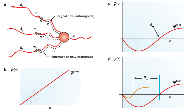
(a) For the information required for Hebbian synaptic modification to be available locally at the synapses, information about the integrated postsynaptic firing rate \(c\) must be propagated backwards or retrogradely. The existence of 'back spiking' (dashed lines) was confirmed experimentally and shown to be associated with changes in synaptic strength.

(b) Simple Hebbian modification assumes that active synapses grow stronger at a rate proportional to the concurrent integrated postsynaptic response; therefore, the value of \(\phi\) increases monotonically with \(c\).

(c) The CLO (Cooper, Liberman, and Oja) theory combined Hebbian and anti-Hebbian learning to obtain a more general rule that can yield selective responses. When a pattern of input activity evokes a postsynaptic response greater than the modification threshold (\(\theta_m\)), the active synapses strengthen; otherwise, the active synapses weaken.

(d) The BCM (Bienenstock, Cooper and Munro) theory incorporates a sliding modification threshold that adjusts as a function of the history of average activity in the postsynaptic neuron. This graph shows the shape of \(\phi\) at two different values of \(\theta_m\). The orange curve shows how synapses modify after a period of postsynaptic inactivity, and the red curve shows how synapses modify after a period of heightened postsynaptic activity.

the important properties of the BCM rule (Intrator and Cooper, 1992)

1. As an exploratory projection index, it seeks deviation from a Gaussian distribution, in the form of multi-modality.
2. It naturally extends to a lateral inhibition network, which can find several projections at once.
3. The number of calculations of the gradient grows linearly with the number of projections sought, thus it is very efficient in high dimensional feature extraction.
4. The search is forced to seek projections that are orthogonal to all but one of the \(K\) clusterings (in the original space). Thus, there are at most \(K\) optimal projections and not \(K(K−1)/2\) separating hyper-planes as in discriminant analysis methods. This property is very important as it suggests why the "curse of dimensionality" is less problematic with this learning rule.
5. [EXTRA] The neuronal output (or the projection) of an input \(x\) (or a cluster of inputs) is proportional to \(1/P(x)\), where \(P(x)\) is the a-priori probability of the input \(x\). This property is (1) essential for creating "suspicious coincidence" detectors, and (2) it also indicates the optimality of the learning rule in terms of energy (or code) conservation. If a biologically plausible logarithmic saturation transfer function is used as the neuronal nonlinearity, it follows that the amplitude or code length associated with the input \(x\) is proportional to \(−\log\left(P\left(x\right)\right)\), which is optimal from information-theoretic considerations.

[some side remarks] Can theory be useful in neuroscience? (Cooper and Bear, 2012)

What is a good theory? The usefulness of a theory lies in its concreteness and in the precision with which questions can be formulated. A successful approach is to find the minimum number of assumptions that imply as logical consequences the qualitative features of the system that we are trying to describe. As Einstein is reputed to have said: “Make things as simple as possible, but no simpler.” Of course there are risks in this approach. We may simplify too much or in the wrong way so that we leave out something essential or we may choose to ignore some facets of the data that distinguished scientists have spent their lifetimes elucidating. Nonetheless, the theoretician must first limit the domain of the investigation: that is, introduce a set of assumptions specific enough to give consequences that can be compared with observation. We must be able to see our way from assumptions to conclusions. The next step is experimental: to assess the validity of the underlying assumptions if possible and to test predicted consequences.

A ‘correct’ theory is not necessarily a good theory. For example, in analysing a system as complicated as a neuron, we must not try to include everything too soon. Theories involving vast numbers of neurons or large numbers of parameters can lead to systems of equations that defy analysis. Their fault is not that what they contain is incorrect, but that they contain too much.

Theoretical analysis is an ongoing attempt to create a structure — changing it when necessary — that finally arrives at consequences consistent with our experience. Indeed, one characteristic of a good theory is that one can modify the structure and know what the consequences will be. From the point of view of an experimentalist, a good theory provides a structure in to which seemingly incongruous data can be incorporated and that suggests new experiments to assess the validity of this structure. A good theory helps the experimentalist to decide which questions are the most important.

lessons?

So, what is it that neurons compute (natively)?

• Do linear algebra (vector projection / inner product, matrix multiplication).
• Implement dimensionality reduction (from many dimensions to one), including similarity-preserving DR by random projections.
• Perform function approximation (when arranged in multilayer networks).
• Respond selectively (exhibit tuning) [and thus serve as landmarks/prototypes in a similarity-based representation scheme, a.k.a. the Chorus Transform].
• Form spatial maps, presumably to facilitate navigation, episodic memory and prospection, and social cognition.
• Form abstract maps (retinotopic, tonotopic, chronotopic, etc.), presumably to facilitate similarity-based readout.
• Organize themselves in dynamic assemblies (note the importance of time) implemented by readout mechanisms.
• Collectively generate oscillating local electrical fields and interact with these fields to implement attention etc.
• Learn.